What is Structural Machine Learning?
Most machine learning tasks are designed for classifying data, but what if you have multiple outcomes? Not only do you have multiple outcomes (Y's or output variables), but you also need to enforce specific relationships among those outcomes and your predictors (X). Traditional ML can do many things, but this is not one of them. Traditional ML classifiers have one outcome and they attempt to classify that univariate outcome.
A genre of machine learning that handles multiple outcomes and allows data scientists to specify a structure among all variables of interest is called "structured prediction". This genre of ML has existed in the literature for many years, but isn't something I've come across much, so I figured I would present a simple form of structured prediction and motivate it with an illustrative example.
The Problem
I'll motivate this with the idea of criminal profiling. It's an interesting subject and something that various researchers and law enforcement entities have been practicing for years. Let's say I want to predict the profile of a criminal offender for a particular offense. We'll define "profile" as the age, sex, race, and residency status (whether or not they live locally) of the offender. Machine learning is data hungry, particularly for more complex models, so we'll need a large data repository for this endeavor. I'll use data from the FBI's NIBRS (National Incidence Based Reporting System) which you can access from this website. You can only download one state at a time. Be aware that you can not download convenient, clean, preformatted data. These downloads contain a slew of tables designed to be a part of a relational database. It also comes with postreSQL code to initialize the tables and load data into them. Consequently, I would recommend using postgres for this task. If you download multiple years or states, you will need to append the data for each state/year to the tables. It would be great if they had a national master file, but that's likely too large. A zipped dump file, maybe? Anyways, just be aware of the format of the data and know you will need to use SQL to get a clean data set.
When it comes to machine learning, python gets most of the love, but I'm an R advocate and will be querying the data and building the model all in R. All code is provided at the very end which includes the data query.
The reason there isn't more out there on structured prediction or libraries that estimate them is that they are very diverse and you can have as many structures as make sense and your data will support. Consequently, they require custom development.
I'm going to skip to the model and problem at hand. For this problem, I have 4 output variables being offender age, sex, race, and residency status. Here a complete Y observation will have four components to it. These are all discrete except age, so I turned it into a discrete variable by creating age categories. The result will have Y-values that look like "M4WR". M = male, 4 = age category 4 (30-39 years), and R = resident. With the way I've categorized the outputs, there are 80 possible categories. 2x5x4x2 = 80. The output space is small enough that we can enumerate them all without much trouble. For many structured prediction problems, enumerating the entire output space is not possible and requires additional work. I'm not going to get into that here, but will try and keep this simple (relatively).
You may ask the question, why then don't we just make this a multi-class classification problem with 80 possible classes? The answer is, you could but that doesn't allow you to specify a structure. In other words, propose various ways of how the variables inter-relate.
Model Structure
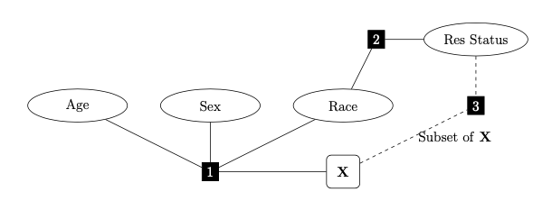
I'm going to specify a relatively simple structure that involves three different "factors" that describe how things relate. I've numbered the factors in the image below so we can keep track of things. Factor 1 is effectively a multi-class classifier with respect to age, sex, and race. That is, we'll be trying to classify 40 different possible combinations of the 3 output variable.

Factor 2 is estimating a relationship between race and residency status. Specifically, it will be producing likelihood scores for each race/residency status combination. Factor 3 will act like a binary classifier because residency status has two outcomes. Resident and non-resident. I separated out residency status because it is a circumstantial attribute rather than a physical one. I think it should be treated separately and I will use different input variables (predictors) to reflect that. I use a subset of the predictor variables regarding the population size of the municipality, and kind of offense, which are the only ones I felt were relevant to a person being a resident. The idea is that there is some domain knowledge about the problem I am attempting to insert into this model through the kind I structure I specify.
In no way am I saying this is the best structure. It merely is a structure, and one I am using to demonstrate a technique.
In the process of prediction, the scores from all three factors will be considered, so there is more going into the decision process than a simple classification procedure. I will be using a structural SVM model for this task. People in stats and data science tend to be familiar with SVMs, and it's a simple one to implement. This uses a structural hinge loss, but nothing would prevent us from using a structural logistic loss, or percpetron loss, and so forth. I implement learning using stochastic gradient descent without any fancy bells or whistles.
For my training and validation samples I use data from 2016-2018, and for the test sample I use criminal incidents from 2019. For validation, I pulled 10% of the data out of the training sample, and use it do quick and dirty tuning of the SVM hyper-parameters.
Results
I got the following results,
- Training performance is about 12% accuracy.
- Validation performance about 13%.
- Test performance about 9%.
As a kind of baseline, the majority label is about 10% of the data. This means test performance is worse than the majority label.
Most people including myself are underwhelmed by this performance. However, the majority of errors involve missing the age or sex components. For example, the true Y-value is M3WR (White, male, age 21-29, resident) and the model predicts M4WR (white male, age 30-39, resident). Most misclassified observations are surprisingly close. Not all of them are close of course, but a good 50% of test sample is a hamming distance of 1 away.
Discussion
I'm not here to defend my illustrative model, though I think it represents a promising first draft of something potentially useful. There are many improvements one could make. The point is to demonstrate structural ML and to motivate its use.
I would also like the reader to consider other reasons why this would not perform well. Perhaps there are some separability concerns with age? Criminal behavior is similar regardless of age (within race, sex, and residency), or certain ages, at least. The test sample is from at least year later. Maybe behavior patterns are not static? Feature engineering is always a thing. Feel free to comment your thoughts to these questions.
It is also worth considering the ethics of using machine learning in this kind of setting. ML has been know to be biased, so these models could easily be racist or sexist, in a way. How would law enforcement or judicial systems react to probabilistic profiling? I bring this up because there are ethical concerns in most worthwhile ML projects. It's not a cure-all and can introduce new problems. I would also like to see people's thoughts regarding the ethics of implementing such a model.
Lastly, I make my code available in case anyone else may find it useful. I believe people seeking knowledge should be able to find it. Thank you for your time, and I hope you enjoyed this post.
Appendix - R Code
----------------------------------------
library(RPostgreSQL)
con<-dbConnect(dbDriver("PostgreSQL"), dbname="utah_nibrs",host="localhost",port="5432")
query<-"SELECT na.data_year AS year, inc.incident_id, arrest_date, na.sex_code AS sex, na.age_num AS age,
nage.age_name AS age_cat, na.resident_code, ag.pub_agency_name AS agency_name, ag.suburban_area_flag AS suburb,
ag.population_group_desc AS pop_cat, ot.offense_name, ot.crime_against, ot.offense_category_name,
inc.incident_hour AS hour,
location_name AS location_type ,rc.race_desc AS race, usel.suspect_using_name AS suspect_using,
vt.victim_type_name, vic.age_num AS victim_age, vnage.age_name AS victim_age_cat, vic.sex_code AS victim_sex, vrc.race_desc AS victim_race,
vic.resident_status_code AS victim_res_status, rel.relationship_name AS vic_off_relationship,
cir.circumstances_name AS circumstances, inj.injury_name AS victim_injury
FROM nibrs_arrestee AS na
INNER JOIN NIBRS_OFFENSE_TYPE AS ot ON (na.offense_type_id = ot.offense_type_id)
INNER JOIN nibrs_age AS nage ON (nage.age_id = na.age_id)
INNER JOIN ref_race AS rc ON (rc.race_id = na.race_id)
INNER JOIN nibrs_incident AS inc ON (na.incident_id = inc.incident_id)
INNER JOIN agencies AS ag ON (inc.agency_id = ag.agency_id)
INNER JOIN nibrs_offense AS ofns ON (na.incident_id = ofns.incident_id)
LEFT JOIN nibrs_suspect_using AS duse ON (ofns.offense_id = duse.offense_id)
LEFT JOIN nibrs_using_list AS usel ON (duse.suspect_using_id = usel.suspect_using_id)
LEFT JOIN nibrs_weapon AS wpid ON (ofns.offense_id = wpid.offense_id)
LEFT JOIN nibrs_weapon_type AS wtyp ON (wpid.weapon_id = wtyp.weapon_id)
INNER JOIN nibrs_location_type lt ON (ofns.location_id = lt.location_id)
-- Join victim data
INNER JOIN nibrs_victim AS vic ON (inc.incident_id = vic.incident_id)
INNER JOIN nibrs_victim_type AS vt ON (vic.victim_type_id = vt.victim_type_id)
INNER JOIN nibrs_age AS vnage ON (vnage.age_id = vic.age_id)
INNER JOIN ref_race AS vrc ON (vrc.race_id = vic.race_id)
LEFT JOIN nibrs_victim_offender_rel AS vor ON (vic.victim_id = vor.victim_id)
LEFT JOIN nibrs_relationship AS rel ON (vor.relationship_id = rel.relationship_id)
LEFT JOIN nibrs_victim_circumstances AS vcr ON (vic.victim_id = vcr.victim_id)
LEFT JOIN nibrs_circumstances AS cir ON (vcr.circumstances_id = cir.circumstances_id)
LEFT JOIN nibrs_victim_injury AS vinj ON (vic.victim_id = vinj.victim_id)
LEFT JOIN nibrs_injury AS inj ON (vinj.injury_id = inj.injury_id)
-- WHERE na.data_year IN (2016,2017,2018)"
nibrs<-dbGetQuery(con,query)
dbDisconnect(con)
rm(con,query)
# quick descriptive summary
age_disc<-dplyr::case_when(nibrs$age <= 17 ~ "Juvenille: <17",
nibrs$age >= 18 & nibrs$age <= 21 ~ "18-21",
nibrs$age >= 22 & nibrs$age <= 29 ~ "22-29",
nibrs$age >= 30 & nibrs$age <= 39 ~ "30-39",
nibrs$age >= 40 & nibrs$age <= 49 ~ "40-49",
nibrs$age >= 50 & nibrs$age <= 65 ~ "50-65",
nibrs$age > 65 ~ "Senior: 65+")
nibrs$age_disc<-factor(age_disc,levels = c("Juvenille: <17","18-21","22-29","30-39","40-49","50-65","Senior: 65+"))
mdat<-nibrs[,-1*c(2,3,5,6,8,13,15,18)]
mdat<-mdat[,c(1:3,9,19,4:8,10:18)]
mdat$tofDay<-dplyr::case_when(mdat$hour >= 5 & mdat$hour < 12 ~ "Morning",
mdat$hour >= 12 & mdat$hour < 17 ~ "Afternoon",
mdat$hour >= 17 & mdat$hour < 22 ~ "Evening",
mdat$hour >= 22 | mdat$hour < 5 ~ "Night",
T ~ "Unknown")
mdat$vic_age_disc<-dplyr::case_when(mdat$victim_age <= 17 ~ "Juvenille: <17",
mdat$victim_age >= 18 & mdat$victim_age <= 21 ~ "18-21",
mdat$victim_age >= 22 & mdat$victim_age <= 29 ~ "22-29",
mdat$victim_age >= 30 & mdat$victim_age <= 39 ~ "30-39",
mdat$victim_age >= 40 & mdat$victim_age <= 49 ~ "40-49",
mdat$victim_age >= 50 & mdat$victim_age <= 65 ~ "50-65",
mdat$victim_age > 65 ~ "Senior: 65+",
T ~ "Unknown")
mdat$vic_age_disc[which(mdat$victim_age_cat=="Over 98 Years Old")]<-"> 98"
mdat$vic_age_disc[which(mdat$victim_age_cat %in% c("1-6 Days Old","7-364 Days Old"))]<-"< 1"
mdat$victim_res_status[which(mdat$victim_res_status==" ")]<-"U"
mdat$vic_off_relationship[is.na(mdat$vic_off_relationship)]<-"Relationship Unknown"
mdat$victim_injury[is.na(mdat$victim_injury)]<-"Unknown"
mdat$circumstances[is.na(mdat$circumstances)]<-"Unknown Circumstances"
mdat<-mdat[,-unique(which(is.na(mdat),arr.ind = T)[,2])]
#mdat$race<-as.factor(mdat$race)
mdat$suburb<-as.factor(mdat$suburb)
mdat$pop_cat<-factor(mdat$pop_cat,levels=c("Cities under 2,500","Cities from 2,500 thru 9,999","Non-MSA counties under 10,000","Cities from 10,000 thru 24,999","Non-MSA counties from 10,000 thru 24,999","MSA counties from 10,000 thru 24,999","Cities from 25,000 thru 49,999","Cities from 50,000 thru 99,999","MSA counties from 25,000 thru 99,999","Cities from 100,000 thru 249,999","MSA counties 100,000 or over"))
mdat$offense_name<-as.factor(mdat$offense_name)
mdat$suspect_using<-as.factor(mdat$suspect_using)
mdat$victim_sex<-as.factor(mdat$victim_sex)
mdat$victim_race<-as.factor(mdat$victim_race)
mdat$victim_res_status<-as.factor(mdat$victim_res_status)
mdat$vic_off_relationship<-as.factor(mdat$vic_off_relationship)
mdat$circumstances<-as.factor(mdat$circumstances)
mdat$victim_injury<-as.factor(mdat$victim_injury)
mdat$tofDay<-factor(mdat$tofDay,level=c("Unknown","Morning","Afternoon","Evening","Night"))
mdat$vic_age_disc<-factor(mdat$vic_age_disc,levels = c("Unknown","< 1","Juvenille: <17","18-21","22-29","30-39","40-49","50-65","Senior: 65+","> 98"))
# get rid of vic age cat
mdat<-mdat[,-11]
cp<-mdat[which(mdat$crime_against=="Person"),]
cp<-cp[-which(cp$resident_code=="U"),]
cp$offense_name<-as.character(cp$offense_name) %>% as.factor()
rm(mdat)
# 1 = American Indian / Alaskan, 2 = Asian, 3 = Black, 4 = Pacific Islander, 5 = Unknown, 6 = White
cp$race<-as.numeric(as.factor(cp$race))
# collapse 1,2,4 as Other -> Other, black, unknown, white
raceSimp<-rep("W",length(cp$race))
raceSimp[which(cp$race %in% c(1,2,4))]<-"O"
raceSimp[which(cp$race == 3)]<-"B"
raceSimp[which(cp$race == 5)]<-"U"
cp$race<-raceSimp
rm(raceSimp)
# numeric values follow levels
cp$age_disc<-as.numeric(cp$age_disc)
# collapse 5-7 to be 40 +
cp$age_disc[which(cp$age_disc>=5)]<-5
# separate to train, validation and test
y<-apply(cp[,c(2,5,4,3)],1, paste,collapse="")
#y<-as.factor(y) %>% as.numeric()
trainy<-y[which(cp$year!=2019)]
trainy<-as.factor(trainy)
testy<-y[which(cp$year==2019)]
testy<-as.factor(testy)
# don't omit reference categories!
x<-model.matrix(~-1+suburb+pop_cat+offense_name+suspect_using+victim_sex+victim_race+victim_res_status+vic_off_relationship+circumstances+victim_injury+tofDay+vic_age_disc,data=cp,contrasts.arg = lapply(cp[,c(6:8,10:18)], contrasts, contrasts=FALSE))
# remove columns that are all zero - consequence of factor variables that are zero once you eliminate unknown residence status
x<-x[,-which(apply(x,2,function(z) all(z==0)))]
trainx<-x[which(cp$year!=2019),]
testx<-x[which(cp$year==2019),]
# validation and training sets
set.seed(23456)
vind<-sample(1:nrow(trainx),size=round(nrow(trainx)*0.1))
# validation sample
vy<-trainy[vind]
vx<-trainx[vind,]
# training sample
trainy<-trainy[-vind]
trainx<-trainx[-vind,]
setdiff(unique(vy),unique(trainy))
setdiff(unique(testy),unique(trainy))
setdiff(unique(trainy),unique(testy))
# remove "F5BN" is it does not exist in the training set
testx<-testx[-which(testy=="F5BN"),]
testy<-testy[-which(testy=="F5BN")]
## Structural SVM - Multi-Class using Kessler Construction ##
yVals<-sort(unique(trainy))
ytoRow<-data.frame(y=yVals,row=1:length(yVals))
AugLoss<-function(x,x3,w1,w2,w3,y,y1toY,y2toY,y3toY,delta,rowLoc,yRowMap,predVals=F){
# Loss Augmented Inference #
score<-array(0,dim=c(nrow(x),nrow(yRowMap),3))
# Factor 1
f1<-x%*%t(w1) # 44796 x 40
for(j in 1:nrow(score)){
for(k in 1:length(y1toY)){
score[j,y1toY[[k]],1]<-f1[j,k]
}
}
# Factor 2 - repeat w2 score vec for all obs
w2row<-rep(0,nrow(yRowMap))
for(j in 1:length(y2toY)){
w2row[y2toY[[j]]]<-w2[j]
}
temp<-matrix(rep(w2row,nrow(score)),nrow=nrow(score),ncol=nrow(yRowMap),byrow = T)
score[,,2]<-temp
# Factor 3
# R = 1, N = -1
#tempy3<-ifelse(substr(ySet[i],4,4)=="R",1,-1)
f3<-(x3%*%w3) # 49773 x 1
score[,y3toY[[1]],3]<-f3
score[,y3toY[[2]],3]<--1*f3
# Loss augmented inference
scrMat<-apply(score,1:2,sum) + delta #element-wise addition
# Compute Loss
maxScore<-apply(scrMat,1,max)
if(predVals){
out<-rep("Oops",length(y))
for(i in 1:length(y)){
out[i]<-yRowMap$y[which(scrMat[i,]==maxScore[i])] %>% as.character()
}
} else {
trueScore<-rep(0,length(y))
for(i in 1:length(y)){
trueScore[i]<-scrMat[i,rowLoc[i]]
}
out<-sum(maxScore-trueScore)
}
return(out)
}
# y mappings to Y outcome space
y1<-substr(ytoRow$y,1,3) %>% unique()
# map y1 to y
y1toY<-lapply(y1,function(z) which(substr(ytoRow$y,1,3) == z))
y2<-substr(ytoRow$y,3,4) %>% unique()
y2toY<-lapply(y2,function(z) which(substr(ytoRow$y,3,4) == z))
y3toY<-lapply(c("R","N"),function(z) which(substr(ytoRow$y,4,4) == z))
# Mapping weight vectors to larger W
Wmap<-matrix(0,nrow(ytoRow),3)
for(j in 1:length(y1toY)){
Wmap[y1toY[[j]],1]<-j
}
for(k in 1:length(y2toY)){
Wmap[y2toY[[k]],2]<-k
}
Wmap[y3toY[[1]],3]<-1
Wmap[y3toY[[2]],3]<--1
strtrSVM<-function(y,x,x3cols,C=100,lr=0.1,tStop=10,yRowMap,Wmap){
# initialize weight and epoch
# w1 corresponds to f1 y_a, y_s, & y_r <-> x ; 2x5x4
w1<-matrix(0,nrow=40,ncol=ncol(x))
# w2 corresponds to y_r <-> y_Res ; 4 x 2 = 8
w2<-rep(0,8)
# w3 corresponds to y_Res <-> x_sub - 65 cols for x_suburb, x_pop_cat, x_offenseName
w3<-rep(0,max(x3cols))
#lossSet<-c(100,hingeLoss(y,x,w))
# establish which W row Map to a given y value
x3<-x[,x3cols]
t<-1
g<-lr/(1+(t-1))
rowLoc<-sapply(y,function(z) yRowMap$row[which(yRowMap$y==z)] )
delta<-sapply(1:length(y),function(z) stringdist::stringdist(y[z],yRowMap$y,method="hamming")) %>% t()
js<-c(C*g*nrow(x),AugLoss(x,x3,w1,w2,w3,y,y1toY,y2toY,y3toY,delta,rowLoc,yRowMap))
# proceed to learning
set.seed(123)
while(t<=tStop){
randInd<-sample(1:nrow(x),replace=T)
xSet<-x[randInd,]
x3Set<-xSet[,x3cols] # hard-coded; limits this to x_suburb, x_pop_cat, and x_offenseName
ySet<-y[randInd]
#if(t %in% seq(0,10000,by=100)) cat("Starting Epoch ",t,"And objective loss is",js[t+1],"\n")
cat("Starting Epoch ",t,"with objective function at",js[t+1],"\n")
for(i in 1:length(y)){
# Inference #
score<-matrix(0,nrow(yRowMap),3)
# Factor 1
f1<-w1%*%xSet[i,] # 40x1 - score for each weight vector
for(j in 1:length(y1toY)){
score[y1toY[[j]],1]<-f1[j]
}
# Factor 2 - w2 is the score - 8x1
for(k in 1:length(y2toY)){
score[y2toY[[k]],2]<-w2[k]
}
# Factor 3
# R = 1, N = -1
#tempy3<-ifelse(substr(ySet[i],4,4)=="R",1,-1)
#f3<-ySet[i]*(w%*%xSet[i,])
score[y3toY[[1]],3]<-(w3%*%x3Set[i,])
score[y3toY[[2]],3]<--1*(w3%*%x3Set[i,])
# Loss augmented inference
yidelta<-stringdist::stringdist(ySet[i],yRowMap$y,method="hamming")
yScore<-apply(score,1,sum) + yidelta
# Max
smax<-max(yScore)
mind<-which(yScore==smax)
gtind<-which(yidelta==0)
# Update Weights #
if(mind[1]==gtind){ # Correct Classification - update margin
wtoUp<-Wmap[gtind,]
# factor 1
w1[wtoUp[1],]<-w1[wtoUp[1],]*(1-g)
# factor 2
w2[wtoUp[2]]<-w2[wtoUp[2]]*(1-g)
# factor 3
w3<-w3*(1-g)
} else { # Incorrect Classification - update weights and margin
wtoUp<-Wmap[union(mind[1],gtind),]
if(nrow(wtoUp) != 2) stop("Wrong Dimension fo wtoUp; gtind must have length of 1")
# factor 1 - multiclass SVM update
# demote wrong decision
w1[wtoUp[1,1],]<-w1[wtoUp[1,1],]*(1-g)-(C*g*xSet[i,])
# promote good decision
w1[wtoUp[2,1],]<-w1[wtoUp[2,1],]*(1-g)-(C*g*-1*xSet[i,])
# factor 2 - y_R & y_Res likelihood score
upy2<-rep(0,length(y2))
upy2[wtoUp[1,2]]<-1
upy2[wtoUp[2,2]]<--1
gvec<-rep(1,length(y2))
# gvec prevents non-updated rows from margin shrinkage
gvec[union(wtoUp[1,2],wtoUp[2,2])]<-1-g
w2<-w2*gvec-(C*g*upy2)
# factor 3 - binary SVM update - update according to incorrect f3
w3<-w3*(1-g)+g*C*wtoUp[1,3]*x3Set[i,]
}
}
t<-t+1
g<-lr/(t)
js<-c(js,AugLoss(x,x3,w1,w2,w3,y,y1toY,y2toY,y3toY,delta,rowLoc,yRowMap))
}
predY<-AugLoss(x,x3,w1,w2,w3,y,y1toY,y2toY,y3toY,delta,rowLoc,yRowMap,predVals = T)
return(list(W=list(w1,w2,w3),pred=predY,objectLoss=js))
}
# y mapping must be in global env
test<-strtrSVM(trainy,trainx,x3cols=1:28,C=10000,lr=0.1,tStop=1000,yRowMap=ytoRow,Wmap=Wmap)
sum(test$pred==trainy)/length(trainy)
# majority label
labfreq<-sort(table(trainy),decreasing=T)
labfreq[1]/length(trainy)
py<-cbind(test$pred,as.character(trainy))
hdist<-stringdist::stringdist(test$pred,trainy,method="hamming")
# most common pred:truth pairs
mistab<-table(apply(py,1,paste,collapse=":")) %>% sort(decreasing=T)


Thank you very much for your post
ReplyDelete