Online Statistics Tutor: Linear Regression - Understanding and Interpreting Linear Regression

Simple Linear Regression is a staple in every statistical toolbox. The idea is to estimate a linear relationship between a dependent variable (Y or your outcome) and an independent variable (X or your predictor variable). That is, we estimate the equation of a line through data points that minimizes the vertical distance of the data points to that line. From this we can better understand how X affects Y. This analysis can be used for predictive purposes, as well.

In this post I plan on only addressing some basic principles about regression in order to best understand what it is and how to use it. I will focus on

• Scatterplots and linear relationships.
• Point-slope equation for a line and how it works.
• Estimating slope coefficients.
• Interpreting the slope.
• Brief mention of other regression concepts (which I may address in later posts). 

Scatterplots and Linear Relationships

If you are not already familiar with what a scatterplot is, it is merely a graphical method to display a bivariate (two-variable) relationship. In simpler terms, we use dots to represent data points and plot them on a graph. The intent here is to be able to discern any pattern in the dots to understand how the independent variable may relate to the dependent variable.

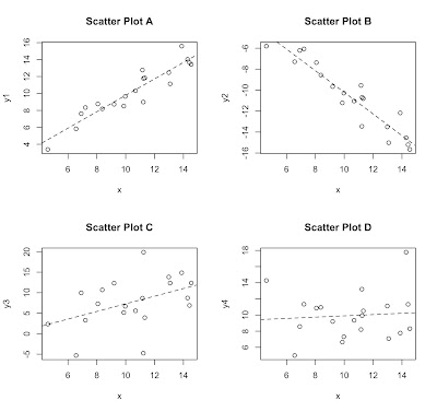
The graphic shows four different scatterplots describing different kinds of linear relationships with a line (a regression line, mind you) highlighting the direction of the relationship. Plots A and B describe strong positive and negative relationships, respectively. I say strong because there is little variation around the line. This mean that X does a good job of explaining what is going on with Y. A positive relationship means that as one variable increases, so does the other. Conversely, a negative relationship means that as one increases, the other decreases. Plot C describes a weaker positive association because the dots are more disperse around the line, meaning that there is more variability in Y that X can not explain. Plot D is essentially flat with no discernible pattern, meaning that there is no relationship. If you have ever learned about correlation coefficients, hopefully this sounds very familiar.

With that crash course in describing numeric relationships in mind, regression is an analysis that provides specific details regarding that linear relationship. Instead of describing a positive or negative relationship, we can say how y changes as x changes. We can also use other statistics involved in regression to assess strength of association.

Point Slope Equation for a Line

To understand the output of a regression model, you'll want to understand or remind yourself of the point-slope form of a line. The generic equation for this form is,

Let's break this down and define all of the elements. y is still your dependent variable and x your independent variable. m represent the slope of the line or the change in y per one unit change in x. b is the y-intercept, which is the value of y when x = 0. Now that we know what that means, let's explain how that works through an example.

The equation for the line in the plot above is y=2x-0.5. Let's start with the y-intercept. Because it is -0.5, we know that the line crosses through (-0.5,0). Let's start our line there. Now we know that the slope is 2, which translates to every time x increases by one, y increases by two. If we were to plot this ourselves we would then start at the y-intercept (-0.5,0) and then go to the right one and then up two and keep doing that. Keep moving to the right 1 and up 2, and you'll have drawn this line.

I bother to do this because understanding the point-slope form of a line will be relevant when you try to interpret your regression output.

Estimating a Regression Line / Slope Coefficient

Regression equations are expressed slightly differently from the point-slope equation.

The latter of the two forms is how you are more likely to see a regression equation expressed, but it is still the same formula for a line. The first coefficient (the beta with the subscript zero) is the intercept, and the second coefficient (beta) is the slope. You are likely noticing that there is an additional term that looks like an E (epsilon). This parameter represents the distance from the individual data points to the regression line and is called the residual error.

To estimate the regression, I will be using R as I do with all my other posts. I'll also be using the UScrime data from the MASS package. To best understand what the regression is doing, I will first demonstrate visually what we are doing before discussing the details. The dependent variable will be the US crime rate and the independent variable will be the GDP. Each point represents a US state.

The estimated regression equation has the same form as the point-slope formula for a line. That's because it is the same thing, and we will interpret it similar to the way that we explained the equation of the line in the last section. The code to do this (including the code I used to make the above graph) in R and the resultant output are provided below.

If you look at the "Estimate" column of the output you see the y-intercept reported as -24.2826 and the slope coefficient for GDP to be 1.7689. Our regression equation for this data is,

Interpreting The Slope Coefficient

Before continuing on, it may help to reread the paragraph that talks about the slope coefficient in the "Point Slope Equation for a Line" section. I'm specifically referring to the paragraph after the line graph. In the example there, we had a slope of two. This means that every time x increased by one, y increases by two. We are going to interpret the slope from our regression equation the same way, however, this time we are going to do so in the context our dependent and independent variables.

When you are interpreting the model output, people are more interested in what the data tells you than what the line looks like. Be sure you understand what the equation tells you about your data. An interpretation for our slope coefficient in terms of our data could go something like, "the regression coefficient of 1.77  estimates that as GDP increases by a value of one, the crime rate is predicted to increase by 1.77". The interpretation I just gave wasn't wildly different from the interpretation of a line, but instead of saying "x" and "y", I used "GDP" and "crime rate".

Additional Regression Concepts

In this post, I only covered regression where there is one predictor or independent variable. You may use as many predictor variables as you want in a regression. This changes the interpretation a bit but not much. It's essentially the same thing, you just have to add "while holding all other coefficients constant" on to the end.

The rabbit hole goes deeper yet. We could still discuss model fit diagnostics, data transformations, higher order terms being non-linear effects and interactions, information criteria, model selection methods, and bayesian methods. Yes, the rabbit hole goes much, much deeper.

I will get to these topics as time permits and where there is the highest demand. If you have interest in any additional regression concepts, don't hesitate to leave a request in the comments.