Online Statistics Tutor: Normal Confidence Intervals - Beginnings of Statistical Uncertainty
This online statistics tutor lesson is intended to supplement introductory statistics material as additional instruction and review. In this lesson we will only be covering beginning concepts regarding confidence intervals around an estimated mean.
Estimating confidence intervals uses essentially the same principles and concepts used for calculating z-scores and normal probabilities (at least for CIs for means estimated from normal data). If you need a refresher regarding these concepts, check out one of my other posts.
The idea behind confidence intervals is to communicate uncertainty regarding our estimates. Here we are taking a step of faith from the theoretical (normal probabilities) to the empirical or observed world. I feel like this is similar to that scene from Indiana Jones and the Last Crusade where he takes "the step of faith". Stepping out into the unseen and unknown and falling upon some substance. In this analogy, that substance would be observed information, being a sample of the phenomenon which we wish to understand better.
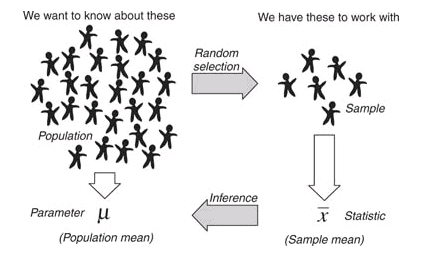
While I could go on, one picture is perhaps worth more than 1,000 words.
Estimating confidence intervals uses essentially the same principles and concepts used for calculating z-scores and normal probabilities (at least for CIs for means estimated from normal data). If you need a refresher regarding these concepts, check out one of my other posts.
Uncertainty in Research and Statistics
Though many are reluctant to admit it, there is a great deal of uncertainty in the information that we consume. Information sources (including legitimate sources) boast new conclusions about the world around us from healthy eating and everyday behavior to climate change and astrophysics. Something that many media sources often glaze over is that NONE of them are 100% sure about their hypothesized conclusion. These conclusions are (hopefully) derived from reliable and representative data, but even under the best of circumstances there is some error. Ideally random error. Ironically, the only conclusion that we are 100% sure of is that we aren't 100% sure.The idea behind confidence intervals is to communicate uncertainty regarding our estimates. Here we are taking a step of faith from the theoretical (normal probabilities) to the empirical or observed world. I feel like this is similar to that scene from Indiana Jones and the Last Crusade where he takes "the step of faith". Stepping out into the unseen and unknown and falling upon some substance. In this analogy, that substance would be observed information, being a sample of the phenomenon which we wish to understand better.
While I could go on, one picture is perhaps worth more than 1,000 words.
It is not realistic for any researcher to observe all instances of the a certain phenomenon. For example, a researcher wanting to know more about the effect of texting on driving can't observe every driver on the planet to see what simultaneous texting does to their driving ability. Consequently, researchers will gather a small sample of people and attempt to test that behavior in a driving simulator.
In a simple situation, and the only one we will discuss here, we attempt to gain knowledge regarding the population (theoretical) mean 𝛍, by calculating the mean from our sample which we denote using x̅. If we take random samples from this population and calculate the mean from each of those samples, we get x̅'s that occur randomly around 𝛍. If sample sizes are large enough, all these different sample means become normally distributed (See Law of Large Numbers; Central Limit Theorem) around the population mean. This normal distribution of sample means is known as the sampling distribution. It is from this sampling distribution that we derive the confidence interval.
The standard deviation of the sampling distribution is known as the standard error. Where the standard deviation is in reference to the raw data, the standard error refers to the sampling distribution, which is made up of estimated means. That is, the standard deviation is composed of X-values, whereas the standard error is made up of x̅'s.
The standard error is calculated by dividing the standard deviation by the square root of the sample size. Which formula can be expressed as,
Example: If we have a sample of 64 and a known standard deviation of 8, what is the standard error of the sampling distribution?
Std Err = 8 / sqrt(64)
Std Err = 8 / 8
Std Err = 1
Nothing terribly difficult there. The confidence interval is composed of different pieces that you are already aware of.
- Estimated Mean
- Standard Error
- Z-score that refers to a specific probability in the standard normal distribution. This probability is often provided as a percent (95%) or as an error rate (alpha = 0.95) This is often referred to as a critical value.
Confidence interval with estimated mean but known Std. Dev.
The formula for a confidence interval for a sample mean is provided below.
These intervals are conventionally expressed as "(lower value, upper value)". When calculating a confidence interval you are given the three pieces of information I mention earlier. Let's go through a simple example to help clear up any confusion.
Example: Please compute a 95% confidence interval for an estimated mean of 5, where 𝝈=2 and n=25.
Let's First establish what are 3 pieces of information are.
- Our estimated mean, x̅ = 5.
- We need to calculate the standard error, and have all of the information we need to do so. The std. err = 2 / sqrt(25) -> = 2 / 5 = 0.4. FYI, I'm just using the formula for the standard error for this.
- Our probability is 0.95 per the expression 95% confidence interval. To do this, we can use a z-table or statistical software (I will use R) to find the central 95% of the area under the normal distribution. Please refer to the post or lesson on normal probabilities, if you don't remember normal probabilities or z-scores. If we are talking about the central 95% (two-tailed) z-score, then that means there is 2.5% of the area beyond the critical z-value. That is because 2.5% on the left and right sides sums to 5%. Be aware that these confidence intervals are, by nature, two tailed.
To get that value out of R we use the function qnorm. The syntax or code for this is
qnorm(0.975, mean=0, sd=1),
which gives us 1.959964. We can round to two decimals place giving us 1.96. This is the same number you will get from a z-table which corresponds to 97.5% of the area, or 2.5% beyond. With all the needed information we are ready to build the confidence interval.
CI = 5±1.96*0.4
upper value = 5 + 1.96*0.4 = 5.784
lower value = 5 - 1.96*0.4 = 4.216
CI = (4.216,5.784)
We are able to use the normal distribution to obtain our critical value because the only source of random error in these examples is coming from an estimated mean. What happens if we have to estimate the standard error as well because the standard deviation for the population must also be estimated?
Confidence intervals when estimating both the mean and standard deviation
If we have to estimate both the mean and the std. dev. then there are two sources of random error and the theoretical normal distribution is no longer appropriate to give us the critical z-score. To account for this addition source of random error, we use the t-distribution which is like the normal distribution but allows for wider intervals when the sample is smaller. Below is a graphic of the t-distribution at different sample sizes or degrees of freedom.
The green line is the t-distribution with a large sample which IS the normal distribution. You can see at lower degrees of freedom this distribution has more area underneath the tails. This makes for wider intervals when we are less sure about or estimates, which I feel is pretty intuitive.
NOTE: If some fellow statistician were to read this page he/she may comment that I have been a bit loose with my formula notation. Which is correct. I have been. This is because the formulae I've given you has a ^ (carat) symbol above 𝛔 which means that the parameter is an estimate. I did this to avoid future confusion about why the formula subtly changes.
Fun fact: when df=1, the t-distribution is the Cauchy distribution and has infinite variance.
What I imagine most students are thinking at this point is, does this make things harder or more complicated? Yes, and no. No, in that you don't really have any additional steps to go through. Yes, in that you have a different table to use to look up critical values.
Let's go back to the same example we did with a known standard deviation that we worked earlier but this time we treat the standard deviation as an estimate. Again,
Example: Please compute a 95% confidence interval for an estimated mean of 5, where sd = 2 and n=25.
Steps one and two don't actually change. The only difference this time is that we will consult a t-table (t-distribution) and not a z-table (normal distribution). Additionally, we need the degrees of freedom for the t-distribution, which is n-1, so not at all difficult to calculate.
CI = 5±t_crit*0.4
To find our critical t-score we must find the score that corresponds to df = 24, consult the t-table or in R we can use qt(0.975,24). We find our critical t-value to be 2.063899 or 2.064 which is what the t-table provides. This changes our confidence interval to,
upper value = 5 + 2.064*0.4 = 5.8256
lower value = 5 - 2.064*0.4 = 4.1744
CI = (4.1744, 5.8256)
That is all the material for this online statistics tutor post. Feel free to request additional topics in the comments. Also, you are welcome to ask me specific questions that you may have regarding this material at this site. In the interest of full disclosure, there is a nominal $1.50 fee to submit questions. That is because it takes time and effort to respond to your questions.
Lesson Glossary
Standard Deviation - The square root of the variance for a sample of data or population.
Standard Error - The standard deviation of the sampling distribution.
Sampling Distribution - The theoretical distribution of parameter estimates (e.g. the mean) built from many numerous samples from the population.
Confidence Interval - An interval with a parameter estimate in the center, which communicates uncertainty regarding that estimate. Specifically, it attempts to address the likelihood of the true population parameter being contained within the interval.
Central Limit Theorem - Mathematical theorem that says the sampling distribution becomes normal for large samples.


Comments
Post a Comment