Beginner Tutorial for Dashboard / Web Development Using R, Shiny, R Markdown.

Creating dashboards is an excellent way to present dynamic and actionable analytic output. There is a plethora of proprietary dashboard software packages but they cost exorbitant amounts to do something that isn't as powerful or flexible as R shiny, which is freely available. Admittedly, many of these software packages provide data / database integration and other bells and whistles, but you can accomplish the same things with a little know how.

My hope is to enable people to produce their desired and perhaps needed dashboard free of cost (other than man hours) without having to commit to a third party vendor. I'll be covering basics here, but if people are also interested in more advanced features such as interactive plots, I can write another tutorial going over that.

I use R Markdown because I find using two R files, one for the UI and the other for the R code (server file) is terribly obnoxious and a bit cumbersome. R Markdown allows you to do it all in one .rmd file. Rstudio has since responded to some of that feedback and has enabled users to develop apps using one app.R file. I still find this a bit clunky and continue using R Markdown. Now don't worry, Rstudio (the company) supports R Markdown in its IDE and will be running all of this in Rstudio (the IDE).

To start, let me provide you with a link on Rstudio's website that takes you through all the shiny widgets and example code for each.  This will likely help answer questions you may be have later on. I also recommend you have this web-document, as well. This "cheat sheet" quickly and effectively communicates how to navigate an Rmarkdown document, its different capabilities, and the syntax to execute them. It's a bit dense with material, but a great guide. If you want to dig through the documentation for the widgets, then go here.

I can't deploy an example dashboard on this website because deploying the dashboard would require an R server to run the R code. Consequently, I'm forced to use screen shots to guide you through this, but if you follow all the steps, you will be able to locally run the resultant .Rmd file in Rstudio. I'll be attaching all my code.

In this post I will be covering

• Opening a new .Rmd document in Rstudio.
• YAML header
• Guide you through the example code automatically provided when you open a new .Rmd file.
• Shiny coding pointers.
• Using R code chunks.
• input calls must be placed inside render functions.

If you have some experience with Rmarkdown and are looking for something beyond the basics, then this particular post is likely not for you. However, I have other posts going over more in depth material. Check those out!

Rstudio's Dashboard Tutorial Code Explanation

For this tutorial, I wanted to first take you through the R Markdown tutorial code the appears every time you open a new file. In a subsequent R markdown tutorial, I will present my own example with more material.

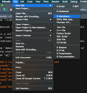
If you do not have Rstudio already, then please download it. Once there, go to New File > R Markdown...

Once you selected that you should see the screen below. The information in the title and author text boxes are placed into your YAML header, but doesn't actually name your file by that title. Just FYI. Be sure to select the Shiny tab on the left.

Once you hit OK, then it will open up a new rmarkdown file that comes with a template file that tries to teach you a few things. It's nice but all this material and far more is covered in the cheat sheet I referenced earlier.

The very top of the document is known as the YAML header. It just provides a header to your html document with the information you provide it along with the desired output. In this case, the output is an html document with runtime as shiny. You can also use R Markdown to produce word documents or latex pdf documents, but that topic is for another time.

The YAML header is done for you if you open a new R Markdown file through R studio. Let's next cover a few basics about the R markdown document.

• plain text becomes plain text in the html document.
• To embed R code in your document follow the example that comes when you open the new document. You only have to do ```{r} to start an R code chunk and then do ``` again to end the R code chunk. Note ` is not an apostrophe rather the key below escape with the ~ (tilde).

The first line in the R code is an inputPanel which is a shiny function for creating a box in which you can place widgets so they look organized. The selectInput and sliderInput are two widgets that the example code use so the user can enter inputs.

Once the inputPanel is complete they then move on to the code that will render the R output. The renderPlot function will render any R graphic, R base graphics, ggplot, or otherwise. You'll likely recognize R's native histogram and empirical density functions that are called within renderPlot. If you compile the document, you will see the output from them if you are unfamiliar with those. These are all the functions that are creating the UI and underlying R code.

Okay, but that isn't everything that's going on, right? How did the widget input information get passed on to the R functions you ask? Well the widget input data is passed by input$widget_title. Input data is stored as a list called "input". You don't see that list created anywhere because it is created behind the scenes when the document gets compiled.

If you look to the line where the hist function is used, at the very end, you will see the syntax input$n_breaks. This is the widget input from the selectInput function. You'll notice that immediately after selectInput there is "n_breaks". This is the name given to that specific widget. So to access that input you'll use input$n_breaks which is exactly what you see in the histogram function's breaks option.

The slider input data is passed to the density function which you see shows up in the adjust option of that function.

A couple things to have in mind.

• input data can only be called within the render functions.
• Consequently, any additional R code that uses input data must be placed within the render function.
• The curly brackets "{}" are used to allow multiple lines of R code to be entered within the render function.

To get your graphic to show up in the html document, be sure that the R code that creates it is in the render function. This may sound obvious, but if you are using ggplot you need to have a line that will produce the graphical object. A line with just object<-ggplot() + geom_whatever() won't cause the graph to appear.

The last section of the Rmarkdown document just pulls another example from some repository which I don't think is at all informative, unless you plan to store your .Rmd file in some repository. That being said, that will be all for this post. Again, if this was too basic for you, I have more posts with more in-depth material.

If you have any specific questions, feel free to ask me at this site. Be aware that there is a nominal $1.50 fee to submit questions. That is because it takes time and effort to respond to your specific questions.

I hope you enjoyed this post and found it helpful. If there is any other R / Rmarkdown related topic you would like to see, feel free to request it in the comments section, or you can pass along any constructive feedback there.